Machine Learning In Stock Trading: An Easy Introduction

Its holiday season. The wifey is out and what better to do than invest time in reviewing some basic application of machine learning applied to the field of Finance. This is a post I have been wanting to write for a long time. All of the Code has been written in R and is easily reproducible. I will not share it here as I dont know how to do it best. Nonetheless the most important packages for achieving this level of black magic are:

1.  Caret
2.  Forecast
3.  Kenrlab
4.  Neuralnet
5.  Xgboost
6.  tseries (sub to PewDiePie)

I will not be reviewing any of the statistical concepts applied but will merely focus on their application and see if we can find any viable/useful results. I feel I should not be saying this as everyon here is a mature adult. BUT this is no financial advice and you should always be doing you due diligence when investing any of your money, not taking advice from a random stranger in the Internet. And bear in mind just because a strategy has worked in the past does not mean it will work in the future.

 

 

 We will be taking a closer look at the share price of the german football behemoth from the Ruhrpott who has been the eternal second after Bayern Munich, Borussia Dortmund.  As can be decuded the share price is highly related to the clubs sporting. So we shouldn’t be expecting too many conclusive results. The stock has also been known to attract some rather peculiar stories as someone bombing the team bus, hoping to hurt members of the staff to financially benefit from it. The time-seris can be seen below. As can be seen the share price has profited from some healthy growth reahcing an all-time high this year.

 

 

But how will proceed? Here a brief overview:

First we will be looking at some feature selection methods such as:

1. Filter Methods
2. Wrapper Methods
3. Embedded Methods

Second we will consider multiple machine learning methods such as:

1. Extreme Gradient Boosting Machine (XGB)
2. Support Vector Machine (SVM)
3. Artifical Neural Networks (ANN)

Third, we will conisder all results and compare them.

After this brief introduction we will finally get our hands dirty. First we will start by simply looking at some feature selection methods. At this point you might be thinking to yourself: “AWWW HELL NAH. JUST SHOW ME HOW TO DO THE THANG” let me tell you that feature selection is one of the most important factors when applying machine learning, so I will briefly run through it. This method consists of simply choosing input predictors. This has multiple advantages such as easy model interpretation, faster learning time, reduced dimensionality and reduced over-fitting. The principal techniques for feature selection are filter, wrapper and ensemble methods.

 

 

Filter methods consist of selecting input predictors based on certain statistical criteria before using them in a learning algorithm.

So first we can try to regress the returns of the share price on themselves using linear regression. Then we can trim down the input predictors down using the p-values. So we lagged the returns up to lag 9 (for no particular reason). Only lag 4 is statistically significant at the 5% level. Nonetheless we will also be looking at lag 3 as it still i statistically significant at level 10%. We have an adjusted r-squared value of 0.006 which is a rather poor result. Hence we will be eliminating all the input predictors unless the aforementioned ones.

 

 

Re-running the linear regression only using lag 3 and lag 4, we get the summary as can be seen below. As we can see re-running the test with less input predictors yields quite different results. The estimates for the single predictors are now different; furthermore, both of the estimates have become more statistically significant. Additionally the Adjusted R-squared has increased, even though still painfully low.

 

 

So we can advance to further ways of selecting our ideal predictor variables. So we can try to find our input predictors wrapper methods. The main advantage of wrappers compared to filter methods is considering interaction with output target features. The downsides of wrapper methods is obviously the increased computational power needed and the risk of over-fitting. Some of the most common Wrapper Methods are:

• Forward selection
• Backward elimination
• Recursive Feature elimination

I personally use backward elimination, where we start with all the features and removes the least significant feature at each iteration which improves the performance of the model. We repeat this until no improvement is observed on removal of features.

 

So using the Caret package we can run this rather simply in R. By the result we can see that the ideal model is composed of four variables, which is able to minimize the mean absolute error (MAE). The lags chosen by the recursive feature selection (rfe) are 4, 5, 1, 7. The results from this little more advanced feature selection is obviously already very different from the results achieved by our simple selection method.

Last but not least we will be looking at embedded methods. These consist of selecting input predictors while using them in learning algorithms and simultaneously maximizing model performance. Embedded methods combine the qualities’ of filter and wrapper methods. It’s implemented by algorithms that have their own built-in feature selection methods. Some of the most popular examples of these methods are LASSO and RIDGE regression which have inbuilt penalization functions to reduce overfitting. I will be using the Lasso regression which performs L1 regularization which adds penalty equivalent to absolute value of the magnitude of coefficients.

Using the Lasso we get a similar result to what we had when we just used the simple linear regression model.

Now that we are done with the feature selection, we can advance to the more juicy stuff.

Going forward we will be using the 4 input predictors we obtained using the recursive feature selection. So this means that we will be using lags 1, 4, 5, 7. Furthermore we will try to run our models via pre-processing our data by using principal component analysis.

So the first machine learning tool we will be using is an Extreme Gradient Boosting (XGB), which is a very commo algorithm (seems to be the favourite from the Kaggle Nerds, joking please don’t boot my nerds). This algorithm is great for supervised learning tasks such as Regression, Classification, and Ranking. EGB has the following parameters.

1. Tree boosting algorithm: it predicts output target feature of weighted sequentially built decision trees
2. Algorithm optimization: it finds local optimal weight coefficients of sequentially built decision trees. For regression, gradient descent algorithm is used for locally minimizing regularized sum of squared errors function, among others.

Running the XGB in R, this is the output we get. So we notice that the number of rounds which minimized our RMSE was 50 and the max tree depth is 1. This can furthermore be observed when looking at the bottom right window, with eta 0.3 and subsample 1. What we could also try (and which I actually did) is to see whether feature extraction via PCA could improve our results.

Principal component analysis (PCA) is a statistical procedure that uses an orthogonal transformation to convert a set of observations of possibly correlated variables (entities each of which takes on various numerical values) into a set of values of linearly uncorrelated variables called principal components. This transformation is defined in such a way that the first principal component has the largest possible variance (that is, accounts for as much of the variability in the data as possible), and each succeeding component in turn has the highest variance possible under the constraint that it is orthogonal to the preceding components.

So quick check if our input predictors are in any shape or form correlated. As we can see none of the input predictors are very much correlated to each other. The most prominent correlation we can observe are at lag 5, which as a positive correlation of 0.08. In this environment using PCA makes not a lot of sense but keep in mind it is a viable tool in a highly correlated environment, such as when checking for interest rate products. Using the PCA pre-processing we finally arrive at an RMSE of 0.02720604 which is actually slightly better than the 0.02723055 RMSE achieved by selection features. Obviously in real-life you would still opt to having as little as possible input predictors. Nonetheless as the results are better and my computer is not suffering too much under the additional computational requirements we will move forward using PCA.

So moving forward, we now will visualize how our residuals behave and try to make sense of our results. Below we can see how our model behaves with respect to the actual time-series of the returns from the share price. The black line represents the actual returns whereas the red line is the estimates from our XGB. You now might be thinking to yourself: “Well this is quite underwhelming…”.

Nonetheless before you rage-quit, keep in mind we want the model to give us directional predictions and not an exact estimate of exactly how much the share price will move. This is exactly what it does, we do not expect the model to reproduce the exact moves of the share, as this would simply mean that the time-series is overfit.

Taking a closer look at the results achieved by the PCA we can see that the results are very similar. Nonetheless the results achieved by pre-processing are much more prominent (simply take my word for this) .

We will now us the model to predict give us a signal and change our position in the stock. We will only consider long or no position, as shorting stocks is just a whole different story.

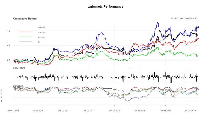
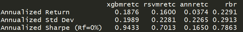
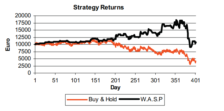
So when running this all we get the following table. The first column “xgbmret” describes simply the returns generated by the model. The second column “xgbmretc” describes the returns generated by the model adjusted for commissions. The commissions were calculated at 10 bps per trade, which actually cuts of fair share or annualized returns. The last column “rbr” simply is the returns generated by a long position. As we can see the model can clearly outperform a simple buy and hold position as it is able to generate higher annualized returns at a much lower risk. Nonetheless the picture changes a little when considering commissions, which place a heavy toll on the performance. When considering any sort of commission, the annualized returns drop by a total of 7 (!!!!!!)percent points. Algebraically it also makes sense that the standard deviation increases. So even though our returns have come down drastically, the Sharpe ratio is still much more performant than a simple buy and hold position.

Furthermore we can check the equity curve to see how the time-series evolved over time. This is useful information as it will help us infer if any of those performances were just lucky at a certain point in time. By looking at the graph we can see that the performance was quite consistent over time. Additionally it allows to infer one of the big advantages of the model, which is the protection against drawdown which the model ensures.

Ok now that we have tested for this model, let us try some other models. I will be proceeding in a similar way but only present you with the results and spare you all the tedious stuff in between.

So next we will be looking at Maximum Margin Methods. These methods consist of supervised boundary based learning algorithms for predicting output target feature by separating output target and input predictor features data into optimal hyper-planes. The most common method for regression learning tasks are support vector machines. Support vector machines are usually used for classification tasks which is obviously our case. Here again we will be using the pre-processed PCA time-series, again because the RMSE is lower. I will spare you most of the previously discussed details. Nonetheless I would like to guide your attention toward this graph below. This graph was already discussed when having a more detailed look at the XGB. What we can see now is that the SVM is more volatile when it comes to projections. So even though it might be more accurate but might cost us more money with respect to commissions we will have to pay.

Here again we can observe what we have observed previously. Nonetheless we can already see that one of the downfalls of the Support Vector Machine is its increased volatility which forces us to change our position many times, forcing us to pay up a lot (hey maybe the broker will send you over some goodies for that). Adjusting for commissions we have to pass on half of our earnings to the broker, which is very hefty. Considering commissions the risk-adjusted performance even becomes worse than the simple Buy and Hold position. This makes clear that it is critical for any signal to be able to blend out random noise. Even though the SVM performed much better than the XGB in an ideal world without commissions, it performed much worse when considering commissions. Now it may be that the commission I am considering is way too high or low, strongly skewing the results. This is the fine balance someone has to consider when setting up any kind of model.

And we can again observe that the trading strategy provides good protection against any sort of downside risk compared to Buy and Hold strategy.

 

Last but not least we will move on to the Artificial Neural Network (ANN), which is part of the Multi-Layer Perceptron Methods. Multi-layer perceptron methods consist of supervised learning algorithms for predicting output target feature by dynamically processing output target and input predictors data through multi-layer network of optimally weighted connections of nodes. The nodes are usually organised in input, hidden and output layers.

In this case we are running the ANN using the features we selected at the beginning. Just to remind you in case of short-term memory loss, these were lag 1, 4, 5, 7. The results, are to say, at the very least very underwhelming. Even though we were able to bring down the standard deviation net or not of commission the returns are just horrendously bad. This obviously does not de-classify the application of ANN, but it just shows that you don’t need the most complicated of machine learning to be able to solve problems related to finance.

So finally we can compare the results of all the algorithms and see which one performed best. When considering the results generated without considering commissions we get see that machine learning algorithms can provide valuable insights. The only machine learning algo which was not able to outperform the Buy and Hold position was the ANN. As previously mentioned the algos are able to provide some existential protection against downside risk. The retuns generated by any of the rules are anyway rather substantial.

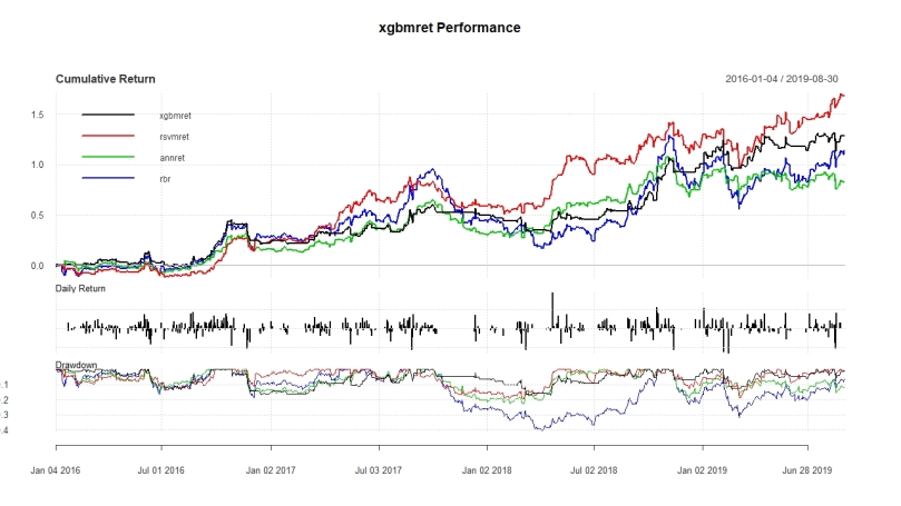
Now ignoring commissions simply is not wise. So the returns worsen a lot when considering commissions. Nontheles we are also able to bring down Std. Dev. drastically, which is a plus. Nonetheless this is still not enough to have a better Sharpe Ratio than the benchmark.

Is the Federal Reserve running out of time?

The Federal Reserve was steamrolled by a perfectly hedged move by the POTUS, who escalated the Chinese tariffs conflict, imposing a 10% tariff on 300 bln of Chinese goods. The POTUS and his team decided to further escalated trade wars, after a calculated move urging the FED to cut the IOER by 50 bps during the FOMC July meeting. Since then the market has rallied to long duration trades, which has led to more curve flattening and further inversion of the 3s10y TSY curve. At this point the 2y10y has still not inverted but has come under massive pressure following recent days. Even though long duration trades are not any novelty, due to the fact that financial institutions are chasing yields at every price possible, the sharp decrease in TSY is astonishing.

Generally a flattening of the curve does not mean a downfall for equities. Nonetheless such a flattening emphasizes the fear of escalating trade wars and a Federal Reserve which is not able to communicate its policy in an effective way. The risk of a market correction/downtrend have risen dramatically and market participants are slowly positioning towards a risk-off scenario, with gold slowly but surely crawling back to the levels of the GFC, trading at USD 1502 with no real profit-taking in sight. The aforementioned global tensions are reflected by equities, most notably the S&P 500, who saw a harsh and quick drawdown. The S&P ended up drawing down 205 points, losing 6.78% of its total market cap.

As of recent the distress is also felt in the interbank market with the 3M LOIS widening back to the yearly high, showing a worsening in credit. The move in credit is widely off-set by liquidity constraints, driving towards a wider the EURUSD XCCY basis. This comes as no surprise with the Treasuries decision of increasing the debt ceiling and the earlier than expected stop in balance sheet unwinding. At this moment the XCCY basis is at some sort of a sweet spot. On the one side Europe investors are looking for high yields in the U.S. zone and on the other side U.S. debt managers are looking at tendering low-yield debt. This can be observed by the growth in reverse Yankee funding.

The 5y5y forward rates on inflation levels have come down from the highs off 2.30 to well below the inflation target of 2% set forth by the Federal Reserve. This comes as an aftermath of the slowing in Economic data and the dovishness of most central banks.

The crucial factors which could impact equities are:

1. Forward Guidance of the Central Banks: As other central banks have proceeded to react to growing worries with respect to global trade tensions, like the RBNZ who cut its rate by 50 bps the FED has come under increasing pressure. Fed Fund Futures are pricing in a total of 100 bps cuts up to December 2020. This is not observable in TSY, where the 2Y Yield is trading at 1.5978. If the Fed is unable to put markets at ease ad keeps running behind the curve we could see a correction in equities. In essence, the September FOMC could be absolutely pivotal to resetting animal spirits. The Fed has plenty of excuses to do this, trade-escalations being the primary factor, particularly as Chair Powell has consistently noted that the biggest risks to the economy are those that are external. Nonetheless compared to the rest of the globe US yields are still very attractive compared to other jurisdiction, like the German 10Y Bund who is yielding at -0,587%.
2. Fading fiscal stimulus: With the fiscal easing under Trump, stocks saw an artificial rejuvenation. Since then fiscal stimulus has faded away and makes the comparison of companies earnings rather difficult. This phenomenon could be observed when fiscal easing began an economic surprise was very high, now with fading effects of fiscal stimulus the Citi Economic Surprise Index has been trending lower.
3. Further Escalation in Trade Wars: In the initial rounds of tariffs President Trump raised tariffs to 25% after having levied an initial 10%. This could well become a deja-vu in the newest round of discussions, between the US and CHINA.

As observed by Citi equity markets seem to be essentially trading like a two-factor model, with the input variables Trump Tweets and FED pricing:

1. The end of 2018 brought about more conciliatory tweets from Trump in November but crucially these were unable to prevent the equity market from correcting ~20% due to a hawkishly delivered Fed hike. An almost immediate dovish turn by Powell in conjunction with a friendly Trump tweet reversed the market sell-off at the turn of the year. At this stage, the money market curve hadn’t yet started to price cuts but did price out further hikes.
2. By the beginning of March stocks were up 18% from the December lows, but an abysmal non-farm payrolls number spooked the money markets into pricing an entire cut by the end of the month. Ironically, this is where the “bad-data = good-news” regime emerged. Data weakness gave lower projected discount rates which helped the equity market rally back to all-time highs in May, supercharged by pacifying Trump tweets.
3. The May escalation of trade wars started the vicious circle of the risk assets relying almost entirely on the premise of Fed cuts. The market recovered as ~70bps worth of Fed cuts were priced by June. Sentiment recovered following what looked like a temporary end to trade escalations in the G20.
4. As of now, the Fed has disappointed the market with a ‘hawkish cut’ whilst there looks to be no sight of trade détente in the short term given the move higher in USD/CNH and the subsequent branding of China as a currency manipulator by the US Administration.

Technical Analysis: Elliott Waves

In todays Weekend Special Edition we will be discussing Elliott Waves. For some technical analytsts Elliott Waves are a vital tool. As any investor the Technical Investor will want to have a reliable forecasting method. The possibility of easy profits by forecasting the market has been the underlying force that motivates so many investors. Elliott’s market model relies heavily on looking at price charts. Practitioners study developing trends to distinguish the waves and waves structures that we will refer to later in this article. The application of the Wave Principle is a form of pattern recognition. To obtain a full understanding of the Wave Principle including the terms and patterns, I recommend Elliott Wave Principle by A.J. Frost and Robert Prechter.

The Elliott Wave Theory was introduced by Ralph Nelson Elliott during the 1930’s. Elliott a full-time accountant believed that stock trends follow a repeating pattern which can be forecasted both in the long and in the short term. The Elliott Wave Theory was published in his book “The Elliott Wave Principle” in 1938. Using data from stocks he concluded that what seems to be a chaotic movement, actually outlines a harmony found in nature. Elliott’s discovery was completely based on empirical data, but he tried to explain his findings using psychological reasons. The main principle of this theory was that a pattern consists of eight waves as can be seen in the Image below.

It is visible that Wave 1, Wave 3 and Wave 5 follow the cyclical trend while waves 2 and 4 correct the underlying trend waves A, B and C correct the overall trend , while Wave A and C follow the correction and Wave B resists. Elliot observed that each wave consists of smaller waves which follow the exact same pattern as is shown in the Image below, thereby forming a super-cycle. The numbers in the Image represent the number of waves when counted in a different scope. For example the whole diagram represents two big waves, the impulse and the correction. The impulse consists of 21 usb-waves which in turn consist of 89 smaller waves, while the Correction wave consists of 13 sub-waves, which in turn, consist of 55 even smaller waves. As can be observed all of the above numbers are part of the Fibonacci series. According to the Elliott wave theory, when Elliott first expressed his theory he was not aware of the Fibonacci series.

Elliot believed that there are nine cycles, of different durations, the bigger of which, is formed by the smaller ones. From the largest to the smallest cycles there are:

1. Grand supercycle: multi-century
2. Super-Cycle: multi-decade (40 to 70 years)
3. Cycle: one year to several years
4. Primary: a few months to a couple of years
5. Intermediate: weeks to months
6. Minor: weeks
7. Minute: days
8. Minuette: hours
9. Subminuette:minutes

The duration of these cycles varies from minutes to decades. Each pattern (cycle) is outlined by the following rules:

1. The Second Wave cannot be longer than the first wave and cannot return to a lower price than that set at the beginning of the first wave
2. The third wave is never the smallest wave compared to the first and the fifth.
3. The fourth wave does not return to a lower price than the price found at the end of the first wave. The same applies for wave a.
4. Usually the third wave shows a greater dynamic, except in some cases where the fifth wave is extended (the case when the fifth wave is made up of five smaller waves)
5. The fifth wave usually leads to a higher point than the third.

When it comes to the interpretation of the waves we will present a short overview of the general dynamic of the waves. The first wave is the “new beginning” of an impulse. Opening a position at this point will be the most profitable scenario. It is difficult to differentiate it from a correction of a previous downtrend, and therefore it is not a powerful wave. Most investors prefer to wait for better timing. The force behind the wave pattern is the number of investors that decide to enter and exit the market at a given time. After some initial winnings, investors decide to exit the market as the price becomes higher, and the stock becomes overpriced for these few investors. This behavior translates in the second wave. As the price begins falling, the stock becomes more attractive for a great number of investors that regretted not having entered the market during the first wave. As the price begins falling, the stock becomes more attractive for a greater number of of investors that regretted not having entered the market at a higher price. Those who entered in the beginning of the wave, are satisfied with their winnings, and have most likely exited the market. Investors realize that the price has reached a level making it difficult to attract any further investors. Demand begins falling, which leads to the fourth wave. Major investors are out of the market, waiting for the end of the fourth wave, to enter again and reap in the profits of the fifth wave. It is important to note that the fourth and the fifth wave are the easiest ones to follow, as they come after the third wave which is the easiest to spot, due to its length, power and speed. Major investors have bought stocks on lower prices, from investors that had bought them during the end of the third wave who feared the price might go lower. However as the major investors enter the market again, they create a small hype, the fifth wave, smaller than the third wave, which usually reaches the peak of the third wave and sometimes even higher. Investors who know the market, know that the market is extremely overrated and therefore have exited the market. Wave A is a corrective wave which is often mistaken for a second wave. This explains wave B. Smaller investors think that wave A corrected the price enough, so that it can lead to an upward trend. Unfortunately, this is the Wave where most smaller, and occasional investors lose huge amounts of money, as Wave C starts, pushing the price lower until the price gets underrated again, for a new pattern to start.

The above explanation is by no means a statistical explanation of the wave behavior, but explains the difference between major and occasional investors and their knowledge of the market. It is exact to know the exact wave patterns , otherwise it is very easy to misinterpret signs. It is important to note that the following explanation regards an overall impulse trend. The opposite would happen in case of an overall correction.

Atsalakis et al (2011) compared the Elliott Wave principle to a Buy and Hold Strategy with remarkable results. The Elliott Wave Principle was tested with the stock of the National Bank of Greece. A paper portfolio worth 10.000 Euros was simulated. Buy and sell decisions did not take into account the confidence index, as it is subjective, depending on the risk the investor is willing to take, even though a threshold of 52% is widely acceptable. Stocks were bought whenever the forecast was positive, and the position was closed when the forecast became negative. Transaction costs were not taken into consideration. The system was tested for period April 2007 to November 2008, for a total of 400 trading days.s. It is worthy to note that this period also includes the great recession of October 2008, were the system achieved interesting results. For the whole period of 400 trading days, the hit rate was 58.75%, mainly due to the crisis. By breaking this period in four sub-periods of 100 observations, the hit rates achieved are 58%, 64%, 60% and 53%, respectively. During this period of 400 trading days, the WASP system made 63 transactions. This gives a rough average of 1 transaction every 6 days.

A beginners guide to Bitcoin investing.

Initial Comments:

So I have decided to post this article as a Weekend Special Edition. Bitcoin is a topic that I have invested a lot of time in myself. This article is a long read for people who really want to try and understand the Bitcoin technology.

As there is no uniform terminology we will refer in this article to Bitcoin as the technology and to bitcoin as the underlying currency itself.

This article will be solely focused on Bitcoin and the underlying Blockchain and is divided in 5 sections:

1. Introduction
2. What is Bitcoin? How does the Blockchain work?
3. Is the Bitcoin setup impenetrable?
4. An empirical analysis on the usage of bitcoins.
5. Valuation of bitcoins

1. Introduction

Bitcoin is a digital currency that creates unique, non-duplicable electronic tokens using software (dubbed mining) with an asymptotic limit of creation of 21 million tokens. Every four years the number of bitcoins created is scheduled to be cut in half until 2040 when creation is supposed to go to zero. The system operates by clearing transactions in a peer-to-peer decentralized system. If you don’t understand the previous sentences, it’a fine as we will come to the core of Bitcoin and the workings of the underlying technology. Since Bitcoin first started trading (on stock exchanges) the 16th of July 2011 the price has increased by baffling 5’209’254% (as of 29.06.2017). Officially Bitcoin was introduced to public in 2009, when Satoshi Nakamoto (allegedly a pseudonym) introduced his whitepaper entitled :”Bitcoin: A Peer-to-Peer Electronic Cash System”.

The bitcoin has enjoyed an enormous increase in valuation, reaching a total market capitalization of 40 billion USD. As shown in the graph above Bitcoin surged for the first time in November of 2013 reaching an all time-high, at a market cap of 13,9 billion USD. Bitcoins plummeted afterwards and hit the floor on a market cap of 2,4 billion USD. On the 11th of June 2017 bitcoins rallied up to a record-breaking 2895,44 USD. Given this recent , nearly unseen rise, it’s astonishing that many people don’t understand what Bitcoins are and how they work. In this article we will try to get to the core of Bitcoin and the underlying blockchain, we will support our assumptions with empirical analysis. One resource will be the whitepaper released by Satoshi Nakamoto. As the concept of Bitcoin is technically complex we will be quoting the most relevant extracts, try to paraphrase them and supplement them with practical examples. If you are a curious and tenacious mind I suggest you read Nakamotos paper yourself.

2. What is Bitcoin? How does the Blockchain work?

“A purely peer-to-peer version of electronic cash would allow online

payments to be sent directly from one party to another without going through a

financial institution.”

This first quote is taken from the abstract and elaborates on the Bitcoins doctrine, a decentralization of cash-flow. Our current methods of making transactions require our money to go through Financial Institutions such as Banks, the FED or any other governmental institution. For years we have trusted financial institutions as middlemen for all of our transactions, the repercussions can be enormous as history has proven. In 2015 Greece was facing a sovereign default, with the Banks having no liquidity and with no re-financing possibilities at first. People were standing on the streets, raiding every ATM they could find in the hopes of saving what was left on their bank deposits. The Greek Government debt crisis has various catalysts, among them a corrupt government and rigged banks. Private Greek banks started according dubious loans and creating a credit bubble that burst in 2010. Two years beforehand Lehman Brothers, a real estate hedge fund disguised as an investment bank, was the originator of the subprime-mortgage financial crisis when it filed for bankruptcy on the 15th of September 2008. By that time, Lehman had assets of $680 billion supported by only $22.5 billion of firm capital. From an equity position, its high risk commercial real estate holdings were three times greater than capital. In such a highly leveraged structure, a three- to five-percent decline in real estate values would wipe out all capital, which finally ended up by happening and causing a financial mayhem . So this really begs the questions: “Why do we entrust banks with our money?”. Because we plain and simply lack alternatives to them. Clearly having all our financial transactions , like loans, credit transactions and savings-account, handled by banks bears a concentration risk. Projects like Kickstarter have been a real alternative to banks, crowdfunding projects thus replacing the process of inquiring for loans at banks. What Nakamoto proposes is that there is a possibility to replace banks as middlemen for online transactions. If we think about electronic money transfer, we have to think this process is just an entry in a register, as no physical cash gets exchanged. If we are able to set-up a public and anonymous register, are we then able to construct an online transaction network without middlemen?

“Commerce on the Internet has come to rely almost exclusively on financial institutions serving as trusted third parties to process electronic payments. While the system works well enough for most transactions, it still suffers from the inherent weaknesses of the trust based model.”

This paragraph extracted from the Introduction accurately pinpoints which problems need to be faced to institute a decentralized network. Nakamoto proposes that the “inherent weaknesses of the trust based model” is a hurdle to online transactions. Completely non-reversible transactions are not possible, since financial institutions cannot avoid mediating disputes. The cost of mediation increases transaction costs, limiting the minimum practical transaction size and cutting off the possibility for small casual transactions. With the possibility of reversal, the need for trust spreads. Merchants must be wary of their customers, hassling them for more information than they would otherwise need. A certain percentage of fraud is accepted as unavoidable. Nakamoto suggests that the trust-model should be replaced by a mathematical model. We will now slowly start to dig into how the blockchain works.

Imagine you are a group of 5 friends sitting in a circle. Everyone in the circle has a sheet of paper and a pen. Friend A wishes to make a 10 euro transaction to friend B. He will now say it out loud and notify the whole group. Everyone in the group verifies if friend A has enough balance to pay friend B and then takes note of the transaction. Whenever enough transactions have been made and documented, all friends put their respective page away in their own folders and start a new one. As you might be able to tell everyone will store away the same amount of information. But before putting away the page, the group of friends needs to make sure that no one can alter the content of what has been documented. The pages need to be sealed with a code that everyone in the group agrees to. In the Bitcoin jargon the process of sealing is defined as mining.

“We define an electronic coin as a chain of digital signatures.”

This is where it starts getting technical. Firstly we will have a closer look at hash functions, as they are the main component of the mining process. A hash function is any function that can be used to map data of arbitrary size to data of fixed size. Suppose you have the number 100 as an argument and run your hash function on it. The output will be “ghakjdhg”. Given our argument that we have now defined as 100. the output will always be the same, in this case “ghakjdhg”. No one will know how your argument got converted into “ghakjdhg” and moreover the process is irreversible, eliminating any possibility of backtracking the functions logic. This means that given the word “ghakjdhg”, it is impossible to tell what our input was, hence why hash functions are very helpful in cryptography. As you might have figured out, hash functions play a role when it comes to Bitcoin mining. To illustrate the usefulness of hash functions in the mining process we will come back to our example with the group of friends. Let’s assume that the total sum of all transactions on one page is equal to 275 Euro, so we label this page with the number 275. Then we will try to find a second number that when added to our number gives us an output of that starts with 4 a`s. After some calculation we may find that this number is 45678. In such a case, 45678 will become the seal for the number 275. To seal the page that bears the sum of 275 euros we will put a badge labeled 45678 on it. An altering of the transaction sum, to lets say 300, would change the output of the hash function. The sealing of numbers is called proof-of-work, as defined in chapter 4 of Nakamotos paper .

“To implement a distributed timestamp server on a peer-to-peer basis, we will need to use a proof-of-work system similar to Adam Back’s Hashcash, rather than newspaper or Usenet posts.The proof-of-work involves scanning for a value that when hashed, […] , the hash begins with a number of zero bits.”

So we have come to the conclusion that the combination of the sealing number and the total sum of transaction gives us a unique output. But who calculates the sealing number? Let’s go back to our group of friends, who has just finished another page of transactions. Everyone in the group engages in the process of calculating a matching sealing number. The first to figure it out will then announce it to the rest of the group. As soon as the sealing number gets announced everyone double-checks if it yields the required output or not.

Some readers now might be asking themselves: “Why should I waste time and energy figuring out a sealing number if eventually someone else might do it?”. This problem gets addressed in Chapter 6, named “Incentive”. Obviously in the real world the process of finding the adequate sealing number, takes up electricity and deteriorates your GPU and/or CPU. The twist is that the first one to calculate the sealing number gets compensated for his success. So imagine we get back to our circle of 5 friends and friend C is able to calculate the sealing number. Friend number C will be rewarded with a freshly printed 1 Euro piece for his efforts, effectively not decreasing anyone’s balance (disregarding any inflationary effects).

We will now advance to digital signatures and how they are embedded in the Bitcoin network. Digital Signatures play a critical role when sending and receiving bitcoins. Digital signatures are the public-key primitives of message authentication. In the physical world handwritten signatures are used to make contracts or documents binding. Similarly, a digital signature is a technique that binds a person or an entity to some sort of digital data and is much less susceptible to fraud.This binding can be independently verified by the receiver as well as any third party. A digital signature is a cryptographic value that is calculated from a secret key, belonging to the signer.

Depicted above we are able to see the flow of a standard normal digital signature process.

Each person involved in the signature flow will have a public and a private key pair. Generally the key pairs used for encryption/decryption and signing/verifying are different. The private key used for signing is referred to as the signature key and the public key as the verification key. The signer feeds some data to a hash function and generates a hash of that data. After obtaining a hash value, its is packed together with the signature key and the package is then fed to the signature algorithm. The algorithm will then proceed to create the digital signature. The signature is appended to the data and both are then sent to the verifier. The verifier then feeds the digital signature and the verification key into the verification algorithm. The verification algorithm gives some values as output, meanwhile the verifier also runs the same hash function on the received data to generate a hash value. This hash value and the output of the verification algorithm are compared. Based on the comparison result, the verifier decides whether the digital signature is valid. The digital signature will be unique, as it is created by the verifier’s private key.

“Each owner transfers the coin to the next by digitally signing a hash of the previous transaction and the public key of the next owner and adding these to the end of the coin. A payee can verify the signatures to verify the chain of ownership.”

To illustrate the Bitcoin transaction procedure we will annex the process flow chart from Nakamotos paper.

For person 1 to transfer a coin to person 2, person 1 signs the hash of the last Bitcoin transaction to occur and the public key of Person 2. Because the network is high-velocity, most of the major parts in the Bitcoin network are high performance supercomputers and dedicated servers that have enough processing power to manage all of the transactions across the continents.

It stands out that bitcoin transactions are very unique in the sense that transactions can be made between parties on opposite sides of the globe via the Internet. Due to the underlying mathematical models no middlemen, such as banks, are needed anymore.

3. Is the Bitcoin setup impenetrable?

While bank robberies and money counterfeiting are of course no problem for an electronic currency, Bitcoin online platforms face severe hacker attacks. Furthermore, due to the lack of regulation the Bitcoin ecosystem remains a “Wild West”. Because Bitcoin transactions are non-revocable, hackers have frequently stolen bitcoins of individuals leaving the victims without recourse. The most common source of scourge to afflict Bitcoin participants has been the denial-of-service attacks (DDoS). These are inexpensive to carry out and quite disruptive. Records show that competing services carry them out in order to improve their market share. A massive DDoS attack hit OKCoin, a China-based Bitcoin exchange, the 10th of July 2015. The platform saw a massive distributed denial of service attack on the which resulted in the international site being shut down for a week. Furthermore the platform compensated traders for losses incurred due to the DDoS. Other times exchanges similar to OKCoin have just shut down without explanation, often with customers losing their deposits. Empirical papers like Vasek et al (2014) show, the number of attacks has increased over time. Böhme et al. (2015) argue that DDoS attacks are especially attractive as stolen Bitcoins can easily be converted into money. We will not dwell into the depths of how such attacks occur but have a look at their frequencies and repercussions. Despite their apparent frequency, very little is known about the true prevalence of DDoS attacks.

From May 2011 to October 2013 142 DDOS attacks on 40 Bitcoin services were documented. Most currency exchanges and mining pools are much more likely to have a DDoS protection such as CloudFlare, Incapsula or Amazon Cloud. Vasek et al (2014) found that 7% of all known operators have been attacked, but that currency exchanges, mining pools, gambling operators, eWallets and financial services are much more likely to be attacked than other services. The study found that big mining pools (those with historical hashrate shares of at least 5%) are much more likely to be DDoSed than small pools.

This Graph issued by Vasek et al. (2014) plots the shift in the DDoS attack targets. We can see that the number and target of reported attacks varies greatly over time. Initially, in the second half of 2011, most DDoS reports concerned mining pools. Then there were very few reported attacks of any kind during the first half of 2012. During the second half of 2012, DDoS attacks picked up again, initially targeting pools, but more frequently targeting currency exchanges and other websites. During 2013, attacks on pools continued, but they were joined by DDoS on gambling websites, eWallets, and currency exchanges. Attacks on currency exchanges dominated the totals from March–June 2013, coinciding with rising exchange rates and unprecedented interest in Bitcoin.

This second table, also published by Vasek et al. (2014), allows a categorisation of DDoS events. Currency exchanges and mining pools make up for nearly 80% of the DDoS attack targets, whereas gambling sites make up for 9%. The figure on the left depicts a cumulative distribution function off how recurrent DDoS attacks are on certain entities. It can be observed that 44% are only attacked once while 15% are attacked on at least on five different occasions. The leader in suffered DDoS attacks was Mt. Gox, with 29 suffered attacks. Mt. Gox was responsible for almost 90% of all the exchange operations in the network before filing for bankruptcy. Mt. Gox has filed for bankruptcy protection from creditors in February of 2014. In April 2014, the company began liquidation proceedings. Out of the 1236 Bitcoin related services only a mere 203 services (16%) have adopted an Anti-DDoS application. The adoption rate among services who have been hit by DDoS attacks is with 54% comparably higher, nonetheless still considerably low.

The Bitcoin’s Proof of work system has been developed to prevent double spending schemes. A double spend attack, is a scheme which enable a certain set of bitcoins to be spent in more than one transaction. Karame et al. (2012) have been able to show that it is possible to bypass the proof of work. While the Bitcoin payment verification process is designed to prevent double spending, Karame et al. show that the system requires tens of minutes to verify a transaction and is therefore inappropriate for fast payments. The security of using Bitcoin for fast payments was analyzed. The paper shows that unless appropriate detection techniques are integrated in the current Bitcoin implementation, doubles spending attacks on fast payments succeed with overwhelming probability and can be mounted at low cost.

4. An empirical analysis on the usage of BTC’s.

We will now take a closer look at what bitcoins are used for and by whom. There are many types of statistics and graphs about the Bitcoin network which can be readily downloaded from the Internet (https://blockchain.info/charts). However these types of statistics tend to describe some global property of the network over time such as the number of daily transactions, their total volume, the number of bitcoins mined so far and the BTCUSD exchange rate. It is very difficult to get accurate information about how bitcoins are used in practice. A paper released in 2013 by Dori Ron and Adi Shamir entitled “Quantitative Analysis of the Full Bitcoin Transaction Graph” provides a detailed understanding off the Bitcoin network . This paper gives a great insight off all transactions from the first time Bitcoins became fully operational up to the 13th of May 2012.The data was gathered from the Bitcoin wallet, which tracks all transactions anonymously Even though the landscape, as of 2012, might have changed this paper provides a great insight towards the typical behaviour of users.

At the time there were 3’730’218 different public keys. 3’120’948 of them were involved as senders in at least one transaction, while the rest of 609’720 appeared to form a network of receivers. One entity (person or company) can have multiple Bitcoin addresses. The paper determined that the total of 3’120’948 addresses can be attributed to 1’851’544 entities. Adding the 1’851’544 entities to the network of receivers only we get a total of 2’460’814 entities involved in the Bitcoins transactions. This implies that on average every entity has 1,5 addresses. However there is a huge statistical variance in the number of addresses an entity manages and in fact one entity is associated with 156’722 different addresses. The paper was able to determine the entity behind all these addresses as being Mt. Gox. The paper made one very interesting finding regarding the distribution of Bitcoins. Of the 9’000’050 bitcoins that were in circulation 7’019’000 bitcoins could be attributed to the 609’720 addresses which only receive and don’t send any bitcoins which were almost 78% of all existing bitcoins. 76.5% of these 78% (or 5’369’535 bitcoins) are what is defined in the paper as “old coins”, this meaning that these coins have not been moved over a time-period of 3 months. The analysis of the total volume of transactions resulted that 40% of all addresses had received fewer than one bitcoin and 59% of the addresses had received fewer than 10 bitcoins over their lifetime. Bitcoin allows for micro transactions, which are called satoshi and are of the order of 10^(-8), this is the smallest fraction into which a bitcoins can be broken up. The paper also goes to show that on the other end of the distribution there was only one address which received over 800’000 bitcoins. The current balance of almost all 98% of all entities was less than 10 bitcoins. 93% percent of all addresses had fewer than 10 transactions each, while 80 addresses used the network for more than 5000 transactions. The paper also goes ahead and dissected the nominal of each transactions. 84% of all the transactions involved fewer than 10 bitcoins. On the other hand large transactions are rare with only 340 transactions larger than 50’000 BTC’s. The paper also went ahead and filtered out 19 of the most active entities. I attached the Table below.

Source

The table shows that Mt. Gox had the most addresses but not the largest accumulated incoming bitcoins nor the largest number of transactions. Six out of the 19 entities have each made fewer than 30 transactions with a total volume of more than 400’000 bitcoins each. A fair conclusion that we can draw from this paper is that most of the mined BTC’s remain dormant in addresses which had never participated in any outgoing transaction. We can also concluded that there is a huge number of tiny transactions which move only a small fraction of a single bitcoin, but there were also hundreds of transactions which moved more than 50’000 bitcoins.

Bitcoin has also been massively linked to the Silk Road in the past, an anonymous, international online marketplace that operates as a Tor hidden service in the past. “More brazen than anything else by light-years” is how U.S. Senator Charles Schumer characterized Silk Road which was shut down March 2015. The Silk road had reportedly between 30’000 and 150’000 active users. The Silk Road was an online “black market” which offered a variety of goods but had a clear focus on drugs. The users were able to stay anonymous, bitcoins granting anonymity even trough the payment process.

5. Valuation of bitcoins

As of now we have only been assessing the design and the technology underlying the decentralized infrastructure of Bitcoin. As this is a financial-centered blog we will try do identify if there are any valuation models for bitcoins. To be able to assess if we can erode a bitcoins value we elaborate whether Bitcoin is primarily an alternative currency or just a speculative asset. According to Kaplanov a currency can be used as a mean of trade, a vehicle to store value, or a unit of account in order to compare the value of different goods or services. Dirk B. et al state that:

“Bitcoin cannot be considered a currency. Its high level of volatility makes a reliable exchange impossible and adversely affects the store of value and unit of account properties. In addition, the fact that it is not an official currency in any country and not backed by any government implies that the high level of volatility affects every Bitcoin transaction, within-country and cross-country transactions. […] Hence, Bitcoin might better be classified as an investment. Its appeal lies in the large historical price movements and expected future returns. Whilst most assets exhibit at least some fluctuations of its price and can thus be labeled risky, Bitcoin appears to be particularly risky and clearly belongs to a high-risk (speculative) asset class.”

Speaking in terms of exchange rates an empirical analysis on volatility shows that minima and maxima observed average daily return for Bitcoin are about 10 times higher than for the Euro or Yen.The standard deviation of realized volatility for the Bitcoin markets varies between 229 and 558 basis points per day, which is 100 times higher than in the FX markets. The Euro FX market exhibits an average of volatility of 50 basis points per day. The figure, published by Dirk B. et al shows that all markets but BTC and Zaydo, from the chosen sample these had the lowest market shares, exhibit moderate statistical skewness. For those two markets the chosen samples show a leptokurtic distribution.

As bitcoins do not provide the feature of an interest rate in contrast to traditional currencies, where interest rates are provided by central banks, valuation models relying on given interest rates are rendered meaningless. Users are left to determine the value of bitcoins themselves by gathering and evaluating information in news and web resources. The price is therefore determined on exchanges by demand and supply. Considering that there is a cap at 21 million bitcoins, as of 8 February 2017 there were 16’152’087,5 bitcoins in circulation, off which many may be lost or not in circulation, it follows that an increasing growth of the demand side is leading to increasing prices. An example how prices can be driven up by an increasing demand can be exemplified with Baidu. On October 14, 2013, Baidu, a web services company that runs the largest search engine in China, began accepting bitcoin. This single action opened the bitcoin network to roughly 570 million internet users in China and prompted other internet companies to consider the cryptocurrency more seriously. The closing price of bitcoin, which averaged just $124 over the 2-week period prior to the announcement, increased to $170 over the 2-week period following the announcement. As we have seen recently the mixture of media attention, the novelty of both the design and the features of a cryptocurrency, combined with its global availability over the internet , have lead to an exponential growth of demand. It seems to be a fair assumption to say that an increase in the number of Bitcoin participants is associated with an increase in the Bitcoin network volume, leading to an increase in the Bitcoin price. It follows that if Bitcoin participants seek to use Bitcoin primarily as an asset, they will not leave a footprint within the Blockchain. This is supported by the common practice of exchanges to keep internal accounts on behalf of their customers. That is, the exchanges are handling accounts of their customers in an internal accounting system, guaranteeing for keeping record of the on-exchange purchased and sold Bitcoins without actually transferring these Bitcoin through the Blockchain. We would expect that those users’ Bitcoins primarily remain within the exchange internal systems.

Users pursuing Bitcoin for its purpose as an alternative asset also lack a valid valuation method. Given that there is no fundamental pricing methodology available, sources of information, like the media, are likely to have a higher influence on prices. Negative news like the announcement of security issues revealed in the underlying protocol should concern users who are using Bitcoin for operational transactions and push some users to re-evaluate the utility and usability and eventually sell their Bitcoin, hence lowering prices on exchanges. Due to the volatile character and the volatile historical prices of the underlying an investor may be aware that they invest in an instrument with a high price uncertainty. Hence, it is a valid assumption that these users only invest a small amount of their total portfolio. They buy Bitcoin at an exchange and store it, waiting for prices to rise. An investor might also keep in mind that if Bitcoin is rendered illegal by change of law, the Bitcoin immediately lose their value. What seems to be noteable is the correlation between the price of Bitcoin and the daily English Bitcoin Wikipedia views, which has been pointed out by Florian Glaser et al. in 2014. This graph helps to identify the mass of particularly uninformed users who have only limited knowledge about Bitcoin and therefore acquire initial information from an initial source of information like Wikipedia.

 

View at Medium.com